Deep Learning2020. 1. 7. 19:54
반응형

 김성훈 교수님의 [모두를 위한 딥러닝] 강의 정리

 - https://www.youtube.com/watch?reload=9&v=BS6O0zOGX4E&feature=youtu.be&list=PLlMkM4tgfjnLSOjrEJN31gZATbcj_MpUm&fbclid=IwAR07UnOxQEOxSKkH6bQ8PzYj2vDop_J0Pbzkg3IVQeQ_zTKcXdNOwaSf_k0

 - 참고자료 : Andrew Ng's ML class

  1) https://class.coursera.org/ml-003/lecture

  2) http://holehouse.org/mlclass/ (note)

  3) http://cs231n.stanford.edu/


1. LeNet-5 [LeCun et al., 1998]

 - 6개의 hidden layer 사용

 ※ softmax에서 좋은 결과를 내기 위한 두 가지 방법 : Deep(layer를 여러 개) & Wide(하나의 layer에 노드를 많이)


2. AlexNet [Krizhevsky et al. 2012]

 - 원본 그림 : 크기 227x227, 색상 RGB 3가지

 - 필터 : 크기 11x11, 개수 96

 - W 개수 : 11x11x3


 - AlexNet 전체 네트워크 구성 : ReLU를 사용한 첫 번째 모델, dropout 및 ensemble도 적용함


3. GoogLeNet [Szegedy et al., 2014]

 - 새로운 이론 'inception module' 적용


4. ResNet [He et al., 2015]

 - 152개의 layer 사용, 2~3주간 8개의 GPU로 학습

 - VGANet(2014년 ImageNet 대회 출전 모델 - 당시 16개의 CONV/FC layer만 사용)보다 빠름


5. ResNet vs GooLeNet


6. CNN for Sentence Classification [Yoon Kim, 2014]


7. AlphaGo [DeepMind]

 - 19x19 크기의 이미지 사용 -> 패딩을 적용하여 23x23 크기로 재구성

 - 48개의 feature planes(채널) 사용 -> 바둑돌 하나 놓을 때마다 48가지 특징으로 판단 (이세돌이 한판이라도 이긴게 대단한 거 아닐까..)

반응형
Posted by CCIBOMB
Deep Learning2020. 1. 3. 23:55
반응형

 김성훈 교수님의 [모두를 위한 딥러닝] 강의 정리

 - https://www.youtube.com/watch?reload=9&v=BS6O0zOGX4E&feature=youtu.be&list=PLlMkM4tgfjnLSOjrEJN31gZATbcj_MpUm&fbclid=IwAR07UnOxQEOxSKkH6bQ8PzYj2vDop_J0Pbzkg3IVQeQ_zTKcXdNOwaSf_k0

 - 참고자료 : Andrew Ng's ML class

  1) https://class.coursera.org/ml-003/lecture

  2) http://holehouse.org/mlclass/ (note)

  3) http://cs231n.stanford.edu/


1. Convolutional Neural Networks (CNN)

 - CONV와 RELU가 한 쌍으로 구성, 중간에 POOL(pooling, sampling, resizing)이 들어감

 - FC : Fully Connected network


2. image로 CNN 이해하기

 (1) Start with an image (width x height x depth)

  - 그림 크기 32 x 32

  - 색상 3가지(red, green, blue) x 3


 (2) Let's focus on a small area only (5 x 5 x 3)

  - 색상에 해당하는 3은 항상 같아야 함


 (3) Get one number using the filter

  - 필터가 차지하는 영역을 하나의 값으로 변환 : Wx + b

  - W는 weight (필터에 해당), x는 외부에서 읽어온 값으로 불변(이미지에 해당)

  - CNN의 목표는 올바른 필터를 찾는 것

  - ReLU 함수를 이용하고 싶다면 간단하게 ReLU(Wx+b)


 (4) Let's look at other areas with the same filter

  - 동일한 필터를 사용하여 다른 영역도 조사


  - 이 때 필터가 움직이는 규칙을 stride라고 하며, ouput의 크기를 계산하면 다음과 같음

    output size = (input size - filter size) / stride + 1


  - 이와 같이 반복되는 경우 convolutional layer를 거칠 때마다 output의 크기가 작아지는 문제가 발생함

    => padding을 통해 해결 (원본이미지 주변을 0으로 채움)


 (5) Swiping the entire image

  - activation map : 여러 개의 필터(convolutional layer)를 거친 출력 결과(channel)


  - activation map(28, 28, 6) :

    output size 28 = (input size 32 - filter size 5) / stride 1 + 1

    filter 개수 6


 (6) Convolutional layers

  - CONV를 거칠 때마다 크기가 작아지고 두꺼워짐

  - 두께는 필터의 개수, 색상, 채널(channel)을 의미함


3. Pooling (sampling, resizing)


 - Max Pooling : 여러 Pooling 기법 중 가장 많이 사용. 여러 개의 값 중 가장 큰 값을 꺼내서 모음


4. FC layer (Fully Connected Layer)

 - 아래 그림의 경우, 최종 결과물이 5개 중 하나 : softmax 사용 


 - CNN 동작을 시각적으로 보여주는 웹사이트 : https://cs.stanford.edu/people/karpathy/convnetjs/demo/cifar10.html


ConvNetJS CIFAR-10 demo


cs.stanford.edu


반응형
Posted by CCIBOMB
Deep Learning2020. 1. 3. 23:39
반응형

 김성훈 교수님의 [모두를 위한 딥러닝] 강의 정리

 - https://www.youtube.com/watch?reload=9&v=BS6O0zOGX4E&feature=youtu.be&list=PLlMkM4tgfjnLSOjrEJN31gZATbcj_MpUm&fbclid=IwAR07UnOxQEOxSKkH6bQ8PzYj2vDop_J0Pbzkg3IVQeQ_zTKcXdNOwaSf_k0

 - 참고자료 : Andrew Ng's ML class

  1) https://class.coursera.org/ml-003/lecture

  2) http://holehouse.org/mlclass/ (note)


1. Softmax classifier for MNIST : Accuracy 0.9035

 - (중요 코드)

# weights & bias for softmax classifier
  hypothesis = tf.matmul(X, W) + b
# define cost/loss & optimizer
  cost = tf.reduce_mean(tf.nn.softmax_cross_entropy_with_logits(logits=hypothesis, labels=Y))
  optimizer = tf.train.AdamOptimizer(learning_rate=learning_rate).minimize(cost)


2. NN for MNIST : Accuracy 0.9455

 - (중요 코드) 3단으로 늘림, ReLU 사용

# weights & bias for nn layers
W1 = tf.Variable(tf.random_normal([784, 256]))
b1 = tf.Variable(tf.random_normal([256]))
L1 = tf.nn.relu(tf.matmul(X, W1) + b1)
 
W2 = tf.Variable(tf.random_normal([256, 256]))
b2 = tf.Variable(tf.random_normal([256]))
L2 = tf.nn.relu(tf.matmul(L1, W2) + b2)
 
W3 = tf.Variable(tf.random_normal([256, 10]))
b3 = tf.Variable(tf.random_normal([10]))
hypothesis = tf.matmul(L2, W3) + b3
 
# define cost/loss & optimizer
cost = tf.reduce_mean(tf.nn.softmax_cross_entropy_with_logits(logits=hypothesis, labels=Y))
optimizer = tf.train.AdamOptimizer(learning_rate=learning_rate).minimize(cost)


3. Xavier Initialization for MNIST (초기화를 잘 하기) : Accuracy 0.9779

 - (중요 코드) 초기값 initializer만 변경

# weights & bias for nn layers
# http://stackoverflow.com/questions/33640581/how-to-do-xavier-initialization-on-tensorflow
W1 = tf.get_variable("W1", shape=[784, 256],
initializer=tf.contrib.layers.xavier_initializer())
b1 = tf.Variable(tf.random_normal([256]))
L1 = tf.nn.relu(tf.matmul(X, W1) + b1)
 
W2 = tf.get_variable("W2", shape=[256, 256],
initializer=tf.contrib.layers.xavier_initializer())
b2 = tf.Variable(tf.random_normal([256]))
L2 = tf.nn.relu(tf.matmul(L1, W2) + b2)
 
W3 = tf.get_variable("W3", shape=[256, 10],
initializer=tf.contrib.layers.xavier_initializer())
b3 = tf.Variable(tf.random_normal([10]))
hypothesis = tf.matmul(L2, W3) + b3


4. Deep NN for MNIST : Accuracy 0.9742 

 - (중요 코드) 5단으로 늘림, 더 넓힘. 깊고 넓게~ => but 결과는 실망 (아마도 overfitting)..

# weights & bias for nn layers
# http://stackoverflow.com/questions/33640581/how-to-do-xavier-initialization-on-tensorflow
W1 = tf.get_variable("W1", shape=[784, 512],
initializer=tf.contrib.layers.xavier_initializer())
b1 = tf.Variable(tf.random_normal([512]))
L1 = tf.nn.relu(tf.matmul(X, W1) + b1)
 
W2 = tf.get_variable("W2", shape=[512, 512],
initializer=tf.contrib.layers.xavier_initializer())
b2 = tf.Variable(tf.random_normal([512]))
L2 = tf.nn.relu(tf.matmul(L1, W2) + b2)
 
W3 = tf.get_variable("W3", shape=[512, 512],
initializer=tf.contrib.layers.xavier_initializer())
b3 = tf.Variable(tf.random_normal([512]))
L3 = tf.nn.relu(tf.matmul(L2, W3) + b3)
 
W4 = tf.get_variable("W4", shape=[512, 512],
initializer=tf.contrib.layers.xavier_initializer())
b4 = tf.Variable(tf.random_normal([512]))
L4 = tf.nn.relu(tf.matmul(L3, W4) + b4)
 
W5 = tf.get_variable("W5", shape=[512, 10],
initializer=tf.contrib.layers.xavier_initializer())
b5 = tf.Variable(tf.random_normal([10]))
hypothesis = tf.matmul(L4, W5) + b5
 
# define cost/loss & optimizer
cost = tf.reduce_mean(tf.nn.softmax_cross_entropy_with_logits(
logits=hypothesis, labels=Y))
optimizer = tf.train.AdamOptimizer(learning_rate=learning_rate).minimize(cost)


5. Dropout for MNIST : Accuracy 0.9804 

 - (중요 코드) 1개의 layer 추가만으로 tensorflow에서 구현 가능. 통상 0.5~0.7로 training 후 1로 testing!

W1 = tf.get_variable("W1", shape=[784, 512], initializer=tf.contrib.layers.xavier_initializer())
b1 = tf.Variable(tf.random_normal([512]))
L1 = tf.nn.relu(tf.matmul(X, W1) + b1)
L1 = tf.nn.dropout(L1, keep_prob=keep_prob)

...

# train my model
for epoch in range(training_epochs):
avg_cost = 0
 
for i in range(total_batch):
batch_xs, batch_ys = mnist.train.next_batch(batch_size)
feed_dict = {X: batch_xs, Y: batch_ys, keep_prob: 0.7}
c, _ = sess.run([cost, optimizer], feed_dict=feed_dict)
avg_cost += c / total_batch
 
print('Epoch:', '%04d' % (epoch + 1), 'cost =', '{:.9f}'.format(avg_cost))
 
print('Learning Finished!')
 
# Test model and check accuracy
correct_prediction = tf.equal(tf.argmax(hypothesis, 1), tf.argmax(Y, 1))
accuracy = tf.reduce_mean(tf.cast(correct_prediction, tf.float32))
print('Accuracy:', sess.run(accuracy, feed_dict={
X: mnist.test.images, Y: mnist.test.labels, keep_prob: 1}))


6. Optimizers

 - GradientDescentOptimizer 外 어떤 알고리즘이 더 좋은지 Simulation 가능

- http://www.denizyuret.com/2015/03/alec-radfords-animations-for.html  


- Adam Optimizer를 처음 써보는 것을 추천 : 기존 코드에서 GradientDescentOptimizer -> AdamOptimizer로만 변경

#define cost/loss & optimizer
cost =tf.reduce_mean(tf.nn.softmax_cross_entropy_with_logits(logits=hypothesis, labels=Y))
optimizer =tf.train.AdamOptimizer(learning_rate=learning_rate).minimize(cost)


반응형
Posted by CCIBOMB
Deep Learning2020. 1. 3. 23:24
반응형

 김성훈 교수님의 [모두를 위한 딥러닝] 강의 정리

 - https://www.youtube.com/watch?reload=9&v=BS6O0zOGX4E&feature=youtu.be&list=PLlMkM4tgfjnLSOjrEJN31gZATbcj_MpUm&fbclid=IwAR07UnOxQEOxSKkH6bQ8PzYj2vDop_J0Pbzkg3IVQeQ_zTKcXdNOwaSf_k0

 - 참고자료 : Andrew Ng's ML class

  1) https://class.coursera.org/ml-003/lecture

  2) http://holehouse.org/mlclass/ (note)


1. Overfitting을 방지하는 3가지 방법

 (1) training data 많이 모으기

  - data가 많은 경우 training set, validation set, test set으로 나누어 진행 가능

  - 영역별 data 크기가 커지므로 overfitting 확률이 낮아짐

 (2) feature 개수 줄이기

  - 서로 비중이 다른 feature가 섞여서 weight 경합시 좋지 않은 결과가 나올 수 있음

  - deep learning은 sigmoid 대신 ReLU 함수를 이용하거나, dropout 등을 통해 해결 가능

 (3) regularization

  - weight이 너무 큰 값을 갖지 않도록 제한


2. Dropout

 - 전체 노드를 weight 계산에 참여시키지 않고, 일부만 참여시키는 아이디어


 - TensorFlow 구현 : relu 함수 호출 후 다음 layer에 전달하기 전 dropout 함수를 호출. 그 비율은 0~1 사이로 랜덤하게.


3. Ensemble (앙상블) :  최소 2%에서 4~5% 상당의 성능 향상을 보임

 1) 데이터를 여러개의 training set으로 나누어 동시에 학습을 진행

 2) 모든 학습이 끝나면 결과를 통합

반응형
Posted by CCIBOMB
Deep Learning2020. 1. 2. 22:30
반응형

 김성훈 교수님의 [모두를 위한 딥러닝] 강의 정리

 - https://www.youtube.com/watch?reload=9&v=BS6O0zOGX4E&feature=youtu.be&list=PLlMkM4tgfjnLSOjrEJN31gZATbcj_MpUm&fbclid=IwAR07UnOxQEOxSKkH6bQ8PzYj2vDop_J0Pbzkg3IVQeQ_zTKcXdNOwaSf_k0

 - 참고자료 : Andrew Ng's ML class

  1) https://class.coursera.org/ml-003/lecture

  2) http://holehouse.org/mlclass/ (note)


1. 모든 wieght 초기값을 0으로 설정한다면,

 - deep learning 알고리즘은 동작하지 않음


2. RBM(Restricted Boltzmann Machine)을 이용한 weight 초기화

 - Hinton et al. (2006) "A Fast Learning Algorightm for Deep Belief Nets" - Restricted Boltzmann Machine

 - Restriction = 같은 layer 안 어떤 연결도 존재하지 않음


 - forward : 현재 layer에 들어온 x값에 대해 weight을 계산한 값을 다음 layer에 전달
   backward : 전달받은 값을 거꾸로 현재 layer에 weight 값을 계산하여 전달

 - forward, backward 계산을 반복하여 최초 전달된 x와 에측한 값(x hat)간 차이가 최소가 되는 weight 발견


 - deep belief net : 이러한 RBM 방식으로 초기화된 모델

 - Fine Tuning : 이러한 방식으로 초기화하여 학습(learning)을 시작하면 시간이 매우 단축됨


3. Xavier/He initialization

 - Xavier : 입력값(fan_in)과 출력값(fan_out) 사이 난수를 선택하여 입력값의 제곱근으로 나눔

 - He : 입력값을 반으로 나눈 제곱급을 사용함. (Xavier보다 넓은 범위의 난수를 생성)


4. 그 밖에 다양한 초기화 방법

반응형
Posted by CCIBOMB
Deep Learning2019. 12. 30. 23:43
반응형

 김성훈 교수님의 [모두를 위한 딥러닝] 강의 정리

 - https://www.youtube.com/watch?reload=9&v=BS6O0zOGX4E&feature=youtu.be&list=PLlMkM4tgfjnLSOjrEJN31gZATbcj_MpUm&fbclid=IwAR07UnOxQEOxSKkH6bQ8PzYj2vDop_J0Pbzkg3IVQeQ_zTKcXdNOwaSf_k0

 - 참고자료 : Andrew Ng's ML class

  1) https://class.coursera.org/ml-003/lecture

  2) http://holehouse.org/mlclass/ (note)


1. Sigmoid

 - Sigmoid 함수는 binary classification에 적절한 함수

 - 처음은 input later, 마지막은 output layer, 가운데 보이지 않는 부분은 hidden layer


 - Vanishing Gradient : 이러한 hidden layer를 2, 3단이 아니라 9, 10단까지 늘릴 경우, 오히려 정확도가 0.5 밖에 되지 않는 문제 발생 : sigmoid 함수가 0~1 사이의 값이므로 이를 9, 10단만큼 곱해지는 경우 거의 0에 수렴하는 작은 값이 되어버림.


2. ReLU (Rectified Linear Unit)

 - Vanishing Gradient를 방지하기 위해, Sigmoid 함수의 개선 함수로 ReLU 함수가 제시됨

 - 0보다 작은 값이 나온 경우 0을 반환하고, 0보다 큰 값이 나온 경우 그 값을 그대로 반환

 - ReLU 구현 :

   함수 max(0, x)

   텐서플로우 적용시에는 sigmoid 함수 대신 relu 함수 사용


3. Sigmoid < ReLU


4. ReLU 외 다양한 활성화 함수들 (Activation Functions)

 - ReLU : max(0, x)처럼 음수에 대해서만 0으로 처리하는 함수
 - Leaky ReLU : ReLU 함수의 변형으로 음수에 대해 1/10로 값을 줄여서 사용하는 함수
 - ELU : ReLU를 0이 아닌 다른 값을 기준으로 사용하는 함수
 - maxout : 두 개의 W와 b 중에서 큰 값이 나온 것을 사용하는 함수
 - tanh : sigmoid 함수를 재활용하기 위한 함수. sigmoid의 범위를 -1에서 1로 넓힘

반응형
Posted by CCIBOMB
Deep Learning2019. 12. 23. 23:43
반응형

 김성훈 교수님의 [모두를 위한 딥러닝] 강의 정리

 - https://www.youtube.com/watch?reload=9&v=BS6O0zOGX4E&feature=youtu.be&list=PLlMkM4tgfjnLSOjrEJN31gZATbcj_MpUm&fbclid=IwAR07UnOxQEOxSKkH6bQ8PzYj2vDop_J0Pbzkg3IVQeQ_zTKcXdNOwaSf_k0

 - 참고자료 : Andrew Ng's ML class

  1) https://class.coursera.org/ml-003/lecture

  2) http://holehouse.org/mlclass/ (note)


1. TensorBoard

 - TensorFlow가 동작하는 방식을 시각화해줌

 - 기존 콘솔방식

 - TensorBoard를 이용한 방식


2. TensorBorad를 이용하기 위한 5가지 단계

 (1) 로그를 남기고 싶은 텐서를 선택

 (2) 한 군데로 모음

 (3) 특정 파일에 기록

 (4) run 함수로 구동한 결과를 add_summary로 추가

 (5) tensorboard 명령으로 결과 확인

   - terminal command line에서 해당 명령어 입력

   - ssh port forwarding을 통해, 원격에서도 확인 가능


3. TensorBorad 실행결과

 - Scalars, Images, Audio, Graphs, Distributions, historgrams, Embeddings 등 확인 가능


4. TensorBoard에서 다양한 조건 실행결과 비교

 - 서로 다른 파일에 로그를 저장하여, 다른 조건에서 실행한 결과를 비교 가능 (ex. learning rate를 달리한 경우)

반응형
Posted by CCIBOMB
Deep Learning2019. 12. 23. 23:02
반응형

 김성훈 교수님의 [모두를 위한 딥러닝] 강의 정리

 - https://www.youtube.com/watch?reload=9&v=BS6O0zOGX4E&feature=youtu.be&list=PLlMkM4tgfjnLSOjrEJN31gZATbcj_MpUm&fbclid=IwAR07UnOxQEOxSKkH6bQ8PzYj2vDop_J0Pbzkg3IVQeQ_zTKcXdNOwaSf_k0

 - 참고자료 : Andrew Ng's ML class

  1) https://class.coursera.org/ml-003/lecture

  2) http://holehouse.org/mlclass/ (note)


1. XOR 알고리즘을 딥러닝으로 풀기 (원리)

 - 논리적으로 매우 간단하지만 초창기 Neural Network에 큰 난관이 됨

 - 하나의 Neural Network unit으로는 XOR 문제를 풀 수 없음 (수학적 증명)

 - 그러나, 여러개의 Neural Network unit으로 XOR 문제 해결이 가능함

 - 위의 unit을 하나로 합쳐서 표시하면, 다음과 같음

 - 여러개의 logistic regression을 하나의 multinomial classification으로 변환 (행렬 이용)

 - 복잡한 네트워크의 weight, bias는 학습이 불가능한 문제가 있었으나, backpropagation으로 해결 가능함

 - 여러 개의 노드들이 있어 복잡한 경우에도 동일함


2. Sigmoid (시그모이드)

 - Logistic regression 또는 Neural network의 Binary classification 마지막 레이어의 활성함수로 사용

 - 시그모이드 함수의 그래프

 - 시그모이드 함수의 미분 (뒤에서부터 순서대로 미분해 나가면 됨)

 - Back propagation 미분을 위한 'TensorFlow'에서의 구현 방식 확인 (TensorBoard에서 확인 가능)


3. XOR 알고리즘을 딥러닝으로 풀기 (TensorFlow 구현)

 (1) XOR 문제를 logistic regression으로 풀기

 - 전체 소스코드

import tensorflow as tf
import numpy as np
 
tf.set_random_seed(777) # for reproducibility
 
x_data = np.array([[0, 0], [0, 1], [1, 0], [1, 1]], dtype=np.float32)
y_data = np.array([[0], [1], [1], [0]], dtype=np.float32)
 
X = tf.placeholder(tf.float32, [None, 2])
Y = tf.placeholder(tf.float32, [None, 1])
 
W = tf.Variable(tf.random_normal([2, 1]), name="weight")
b = tf.Variable(tf.random_normal([1]), name="bias")
 
# Hypothesis using sigmoid: tf.div(1., 1. + tf.exp(tf.matmul(X, W)))
hypothesis = tf.sigmoid(tf.matmul(X, W) + b)
 
# cost/loss function
cost = -tf.reduce_mean(Y * tf.log(hypothesis) + (1 - Y) * tf.log(1 - hypothesis))
train = tf.train.GradientDescentOptimizer(learning_rate=0.1).minimize(cost)
 
# Accuracy computation
# True if hypothesis>0.5 else False
predicted = tf.cast(hypothesis > 0.5, dtype=tf.float32)
accuracy = tf.reduce_mean(tf.cast(tf.equal(predicted, Y), dtype=tf.float32))
 
# Launch graph
with tf.Session() as sess:
# Initialize TensorFlow variables
sess.run(tf.global_variables_initializer())
 
for step in range(10001):
_, cost_val, w_val = sess.run(
[train, cost, W], feed_dict={X: x_data, Y: y_data}
)
if step % 100 == 0:
print(step, cost_val, w_val)
 
# Accuracy report
h, c, a = sess.run(
[hypothesis, predicted, accuracy], feed_dict={X: x_data, Y: y_data}
)
print("\nHypothesis: ", h, "\nCorrect: ", c, "\nAccuracy: ", a)


 - 결과값

Hypothesis: [[ 0.5]
[ 0.5]
[ 0.5]
[ 0.5]]
Correct: [[ 0.]
[ 0.]
[ 0.]
[ 0.]]
Accuracy: 0.5


 (2) XOR 문제를 Neural Net으로 풀기

 - 기존의 소스코드와 동일하나 L1, W2, b2 부분 유의

 - 상기 부분만 수정하였음에도 정확도가 100%로 향상됨

 - 전체 소스코드

import tensorflow as tf
import numpy as np
 
tf.set_random_seed(777) # for reproducibility
 
x_data = np.array([[0, 0], [0, 1], [1, 0], [1, 1]], dtype=np.float32)
y_data = np.array([[0], [1], [1], [0]], dtype=np.float32)
 
X = tf.placeholder(tf.float32, [None, 2])
Y = tf.placeholder(tf.float32, [None, 1])
 
W1 = tf.Variable(tf.random_normal([2, 2]), name='weight1')
b1 = tf.Variable(tf.random_normal([2]), name='bias1')
layer1 = tf.sigmoid(tf.matmul(X, W1) + b1)
 
W2 = tf.Variable(tf.random_normal([2, 1]), name='weight2')
b2 = tf.Variable(tf.random_normal([1]), name='bias2')
hypothesis = tf.sigmoid(tf.matmul(layer1, W2) + b2)
 
# cost/loss function
cost = -tf.reduce_mean(Y * tf.log(hypothesis) + (1 - Y) * tf.log(1 - hypothesis))
train = tf.train.GradientDescentOptimizer(learning_rate=0.1).minimize(cost)
 
# Accuracy computation
# True if hypothesis>0.5 else False
predicted = tf.cast(hypothesis > 0.5, dtype=tf.float32)
accuracy = tf.reduce_mean(tf.cast(tf.equal(predicted, Y), dtype=tf.float32))
 
# Launch graph
with tf.Session() as sess:
# Initialize TensorFlow variables
sess.run(tf.global_variables_initializer())
 
for step in range(10001):
_, cost_val = sess.run([train, cost], feed_dict={X: x_data, Y: y_data})
if step % 100 == 0:
print(step, cost_val)
 
# Accuracy report
h, p, a = sess.run(
[hypothesis, predicted, accuracy], feed_dict={X: x_data, Y: y_data}
)
 
print(f"\nHypothesis:\n{h} \nPredicted:\n{p} \nAccuracy:\n{a}")


 - 결과값

Hypothesis:
[[0.01338216]
[0.98166394]
[0.98809403]
[0.01135799]]
Predicted:
[[0.]
[1.]
[1.]
[0.]]
Accuracy:
1.0
'''


 (3) XOR 문제를 Wide Neural Net으로 풀기

 - Layer의 입력값이 많아지도록 하여, 이미지의 출력값을 증가시킴 -> Hypothesis가 향상됨 (Cost가 줄어듬)

 - Wide하거나 Deep하게 학습을 시키는 경우 Cost 값이 대부분 작아짐

 - 그러나 너무 잘 맞게 학습되는 경우, Overfitting 현상이 발생 가능함


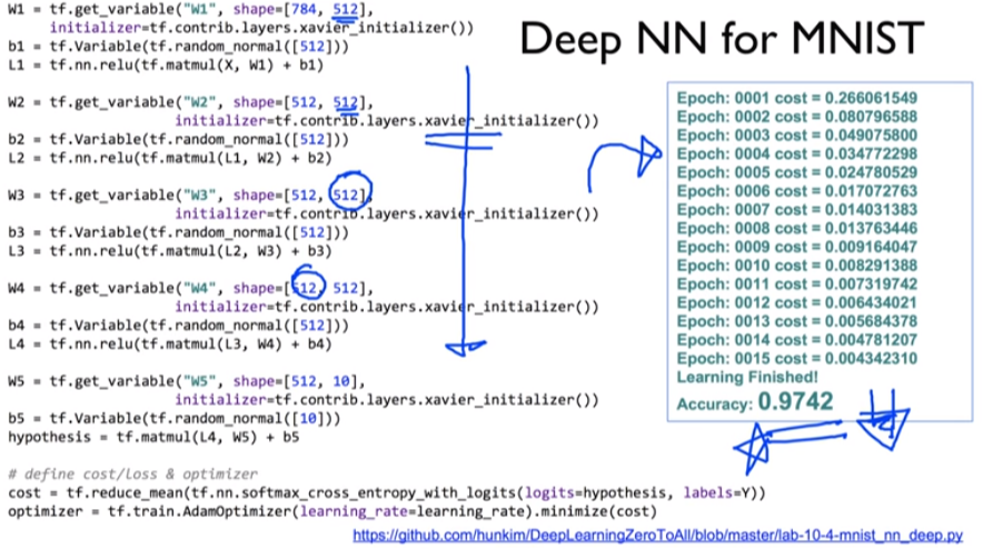
 (4) XOR 문제를 Deep Neural Net으로 풀기

 - NN과 동일한 방법으로 단계를 여러번 반복함


반응형
Posted by CCIBOMB
Deep Learning2019. 12. 18. 23:04
반응형

 김성훈 교수님의 [모두를 위한 딥러닝] 강의 정리

 - https://www.youtube.com/watch?reload=9&v=BS6O0zOGX4E&feature=youtu.be&list=PLlMkM4tgfjnLSOjrEJN31gZATbcj_MpUm&fbclid=IwAR07UnOxQEOxSKkH6bQ8PzYj2vDop_J0Pbzkg3IVQeQ_zTKcXdNOwaSf_k0

 - 참고자료 : Andrew Ng's ML class

  1) https://class.coursera.org/ml-003/lecture

  2) http://holehouse.org/mlclass/ (note)


1. Shape, Rank, Axis

 - Rank : 행렬의 차원(dimension). 1차원인 경우 1, 2차원인 경우 2.

            대괄호 '['의 개수를 세면 됨

 - Axis : 축. 가장 바깥 대괄호의 axis = 0 가장 안쪽의 axis = rank -1

 - Shape : 행렬의 구조. 행렬 형태의 표시방법(행렬츼 차원 및 요소가 몇개인지)


2. Broadcasting # 사용시 유의!


3. Reduce mean, Reduce sum

 - integer 인지 float 인지에 따라 결과값 달라짐을 주의해야 함

 - axis(축)에 따라 결과값 달라짐도 주의해야 함


4. Argmax

 - 가장 큰 값이 있는 위치를 구함


5. Reshape

 - reshape은 원하는 shape를 직접 입력하여 바꿀 수 있음

 - shape에 -1을 입력하면 고정된 차원을 채우고 남은 부분을 알아서 채워줌


 - Reshape (squeeze, expand)

   squeeze : 차원 중 사이즈가 1인 것을 찾아 스칼라값으로 바꿔 해당 차원을 제거함

   expand_dims : axis로 지정된 차원을 추가함


6. One hot

 - 입력받은 행렬보다 마지막에 한차원이 증가함

 - reshape을 통해 다시 증가한 차원을 줄여줄 수 있음 


7. Casting

 - Tensor를 새로운 형태로 캐스팅하는데 사용함

 - 부동소수점형(float)에서 정수형(int)으로 바꾼 경우 소수점 버림

 - Boolean 형태인 경우 True이면 1, False이면 0을 반환


8. Stack

 - 여러 조각의 행렬을 합침

 - axis = 0 / axis = 1에 따라 stack을 쌓는 방식이 달라짐


9. ones_like, leros_like

 - 주어진 shape과 동일하게 0 또는 1을 채운 행렬을 만듦


10. Zip

 - 여러 개의 Tensor를 한번에 추출

반응형
Posted by CCIBOMB
Deep Learning2019. 12. 18. 22:28
반응형

 김성훈 교수님의 [모두를 위한 딥러닝] 강의 정리

 - https://www.youtube.com/watch?reload=9&v=BS6O0zOGX4E&feature=youtu.be&list=PLlMkM4tgfjnLSOjrEJN31gZATbcj_MpUm&fbclid=IwAR07UnOxQEOxSKkH6bQ8PzYj2vDop_J0Pbzkg3IVQeQ_zTKcXdNOwaSf_k0

 - 참고자료 : Andrew Ng's ML class

  1) https://class.coursera.org/ml-003/lecture

  2) http://holehouse.org/mlclass/ (note)


1. MNIST Dataset

 - 숫자 0~9까지의 손글씨 이미지의 집합

 - 학습데이터 60,000개, 테스트데이터 10,000개로 구성

 - 사이즈는 28 x 28, 이미지의 값은 0 또는 1 (흑 또는 백)

 - preprocessing, formatting이 모두 완료된 데이터셋

 - 다운로드 주소 : http://yann.lecun.com/exdb/mnist/


2. TensorFlow에서 MNIST Dataset 불러오기 using input_data.py

 - 다운로드 주소 : https://github.com/tensorflow/tensorflow/blob/r0.7/tensorflow/examples/tutorials/mnist/input_data.py

from tensorflow.examples.tutorials.mnist import input_data
 
# Check out https://www.tensorflow.org/get_started/mnist/beginners for
# more information about the mnist dataset
mnist = input_data.read_data_sets("MNIST_data/", one_hot=True)
 
nb_classes = 10
 
# MNIST data image of shape 28 * 28 = 784
X = tf.placeholder(tf.float32, [None, 784])
# 0 - 9 digits recognition = 10 classes
Y = tf.placeholder(tf.float32, [None, nb_classes])
 
W = tf.Variable(tf.random_normal([784, nb_classes]))
b = tf.Variable(tf.random_normal([nb_classes]))


3. Softmax

# Hypothesis (using softmax)
hypothesis = tf.nn.softmax(tf.matmul(X, W) + b)
 
cost = tf.reduce_mean(-tf.reduce_sum(Y * tf.log(hypothesis), axis=1))
train = tf.train.GradientDescentOptimizer(learning_rate=0.1).minimize(cost)
 
# Test model
is_correct = tf.equal(tf.argmax(hypothesis, 1), tf.argmax(Y, 1))
# Calculate accuracy
accuracy = tf.reduce_mean(tf.cast(is_correct, tf.float32))


4. Training epoch/batch

 - epoch : 전체 training set을 1회 학습

 - batch : 1 epoch을 나누어서 실행하기 위한 사이즈

# parameters
num_epochs = 15
batch_size = 100
num_iterations = int(mnist.train.num_examples / batch_size)
 
with tf.Session() as sess:
# Initialize TensorFlow variables
sess.run(tf.global_variables_initializer())
# Training cycle
for epoch in range(num_epochs):
avg_cost = 0
 
for i in range(num_iterations):
batch_xs, batch_ys = mnist.train.next_batch(batch_size)
_, cost_val = sess.run([train, cost], feed_dict={X: batch_xs, Y: batch_ys})
avg_cost += cost_val / num_iterations
 
print("Epoch: {:04d}, Cost: {:.9f}".format(epoch + 1, avg_cost))
 
print("Learning finished")


5. Report results on test dataset

# Test the model using test sets
print(
"Accuracy: ",
accuracy.eval(
session=sess, feed_dict={X: mnist.test.images, Y: mnist.test.labels}
),
)


6. Sample image show and prediction

# Get one and predict
r = random.randint(0, mnist.test.num_examples - 1)
print("Label: ", sess.run(tf.argmax(mnist.test.labels[r : r + 1], 1)))
print(
"Prediction: ",
sess.run(tf.argmax(hypothesis, 1), feed_dict={X: mnist.test.images[r : r + 1]}),
)
 
plt.imshow(
mnist.test.images[r : r + 1].reshape(28, 28),
cmap="Greys",
interpolation="nearest",
)
plt.show()


7. 전체 소스코드

import tensorflow as tf
import matplotlib.pyplot as plt  # matplotlib : 이미지를 다루는 라이브러리
import random  # random : W와 b에 임의 값을 주는 역할
 
tf.set_random_seed(777) # for reproducibility
 
from tensorflow.examples.tutorials.mnist import input_data
 
# Check out https://www.tensorflow.org/get_started/mnist/beginners for
# more information about the mnist dataset
mnist = input_data.read_data_sets("MNIST_data/", one_hot=True)  # MNIST Dataset 다운로드
 
nb_classes = 10  # 10개 label(0~9) 분류
 
# MNIST data image of shape 28 * 28 = 784 (이미지 feature 784개)
X = tf.placeholder(tf.float32, [None, 784])
# 0 - 9 digits recognition = 10 classes (이미지와 매칭되어 있는 label(정답) 10종류)
Y = tf.placeholder(tf.float32, [None, nb_classes])
 
W = tf.Variable(tf.random_normal([784, nb_classes]))  # W, b : 랜덤으로 값 지정
b = tf.Variable(tf.random_normal([nb_classes]))
 
# Hypothesis (using softmax)
hypothesis = tf.nn.softmax(tf.matmul(X, W) + b)  # 가설함수 H(X)를 softmax에 대입
 
cost = tf.reduce_mean(-tf.reduce_sum(Y * tf.log(hypothesis), axis=1))  # Cross-Entropy를 이용한 cost
train = tf.train.GradientDescentOptimizer(learning_rate=0.1).minimize(cost)  # Gradient Descent Algorithm을 이용한 cost 최소화
 
# Test model : 정답(label)과 H(X)의 예상결과 비교
is_correct = tf.equal(tf.argmax(hypothesis, 1), tf.argmax(Y, 1))
# Calculate accuracy : 정확도 측정
accuracy = tf.reduce_mean(tf.cast(is_correct, tf.float32))
 
# parameters
num_epochs = 15  # 전체 이미지를 15회 반복 학습
batch_size = 100  # 학습 이미지 파일이 많아서 100개씩 가져옴
num_iterations = int(mnist.train.num_examples / batch_size)
 
with tf.Session() as sess:
# Initialize TensorFlow variables : TensorFlow 변수 초기화 및 세션 시작
sess.run(tf.global_variables_initializer())
# Training cycle
for epoch in range(num_epochs):
avg_cost = 0
 
for i in range(num_iterations):
batch_xs, batch_ys = mnist.train.next_batch(batch_size)  # Training 데이터를 X와 Y에 너헝줌
_, cost_val = sess.run([train, cost], feed_dict={X: batch_xs, Y: batch_ys})  # 학습과정의 cost 계산
avg_cost += cost_val / num_iterations
 
print("Epoch: {:04d}, Cost: {:.9f}".format(epoch + 1, avg_cost))  # 1회 학습당 cost 결과 출력
 
print("Learning finished")
 
# Test the model using test sets : Test 데이터를 이용하여 label(정답)과 비교. 정확도 계산
print(
"Accuracy: ",
accuracy.eval(
session=sess, feed_dict={X: mnist.test.images, Y: mnist.test.labels}
),
)
 
# Get one and predict
r = random.randint(0, mnist.test.num_examples - 1)  # Test 데이터에서 임의의 값을 뽑아서 예측
print("Label: ", sess.run(tf.argmax(mnist.test.labels[r : r + 1], 1)))
print(
"Prediction: ",
sess.run(tf.argmax(hypothesis, 1), feed_dict={X: mnist.test.images[r : r + 1]}),
)
 
plt.imshow(
mnist.test.images[r : r + 1].reshape(28, 28),
cmap="Greys",
interpolation="nearest",
)
plt.show()  # Test 데이터에서 뽑은 이미지 출력


반응형
Posted by CCIBOMB