※ 김성훈 교수님의 [모두를 위한 딥러닝] 강의 정리
- 참고자료 : Andrew Ng's ML class
1) https://class.coursera.org/ml-003/lecture
2) http://holehouse.org/mlclass/ (note)
1. Hypothesis and Cost
- 기존 Hypothesis and Cost

- 단순화한 Hypothesis and Cost

2. Gradient descent algorithm
- cost 최소화 등 많은 최소화 문제 해결에 활용되는 알고리즘
- cost(W,b)의 경우, cost를 최소화하는 W, b 값을 찾아냄
- 미분을 하여 기울기가 최소가 되는 점이 cost가 최소가 되는 점
- linear regression을 사용할 때, cost function이 convex function(볼록함수)이 되는지 확인해야 함
-> 그래야 정확한 값 획득 가능

3. Linear Regression의 cost 최소화의 Tensorflow 구현
| import tensorflow as tf |
| import matplotlib.pyplot as plt // "pip install matplotlib" 명령어 실행을 통해 사전 설치 필요 (그래프 그려주는 라이브러리) |
| X = [1, 2, 3] |
| Y = [1, 2, 3] |
| W = tf.placeholder(tf.float32) |
| # Our hypothesis for linear model X * W |
| hypothesis = X * W |
| # cost/loss function |
| cost = tf.reduce_mean(tf.square(hypothesis - Y)) |
| # Variables for plotting cost function |
| W_history = [] |
| cost_history = [] |
| # Launch the graph in a session. |
| with tf.Session() as sess: |
| for i in range(-30, 50): |
| curr_W = i * 0.1 |
| curr_cost = sess.run(cost, feed_dict={W: curr_W}) |
| W_history.append(curr_W) |
| cost_history.append(curr_cost) |
| # Show the cost function |
| plt.plot(W_history, cost_history) |
| plt.show() |

4. Gradient descent algorithm 적용

(1) 미분을 이용한 알고리즘 수동 구현
| # Minimize: Gradient Descent using derivative: W -= learning_rate * derivative |
| learning_rate = 0.1 // 알파 값 |
| gradient = tf.reduce_mean((W * X - Y) * X) |
| descent = W - learning_rate * gradient |
| update = W.assign(descent) |
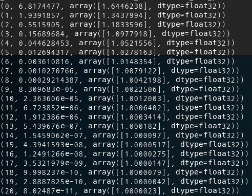
- full code
| import tensorflow as tf |
| tf.set_random_seed(777) # for reproducibility |
| x_data = [1, 2, 3] |
| y_data = [1, 2, 3] |
| # Try to find values for W and b to compute y_data = W * x_data |
| # We know that W should be 1 |
| # But let's use TensorFlow to figure it out |
| W = tf.Variable(tf.random_normal([1]), name="weight") |
| X = tf.placeholder(tf.float32) |
| Y = tf.placeholder(tf.float32) |
| # Our hypothesis for linear model X * W |
| hypothesis = X * W |
| # cost/loss function |
| cost = tf.reduce_mean(tf.square(hypothesis - Y)) |
| # Minimize: Gradient Descent using derivative: W -= learning_rate * derivative |
| learning_rate = 0.1 |
| gradient = tf.reduce_mean((W * X - Y) * X) |
| descent = W - learning_rate * gradient |
| update = W.assign(descent) |
| # Launch the graph in a session. |
| with tf.Session() as sess: |
| # Initializes global variables in the graph. |
| sess.run(tf.global_variables_initializer()) |
| for step in range(21): |
| _, cost_val, W_val = sess.run( |
| [update, cost, W], feed_dict={X: x_data, Y: y_data} |
| ) |
| print(step, cost_val, W_val) |
(2) 텐서플로우의 Optimizer를 이용한 구현 (굳이 우리가 직접 미분하지 않아도 됨)
| #Minimize: Gradient Descent Magic |
| optimizer = tf.train.GradientDescentOptimizer(learning_rate=0.1) |
| train = optimizer.minimize(cost) |
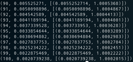
- full code
import tensorflow as tf
tf.set_random_seed(777) # for reproducibility
# tf Graph Input
X = [1, 2, 3]
Y = [1, 2, 3]
W = tf.Variable(tf.random_normal([1], name="weight"))
# Linear model
hypothesis = X * W
# cost/loss function
cost = tf.reduce_mean(tf.square(hypothesis - Y))
# Minimize: Gradient Descent Optimizer
train = tf.train.GradientDescentOptimizer(learning_rate=0.1).minimize(cost)
# Launch the graph in a session.
sess = tf.Session()
# Initializes global variables in the graph.
sess.run(tf.global_variables_initializer())
for step in range(101):
_, W_val = sess.run([train, W])
print(step, W_val)

- W 초기값을 5로 주었을 때,
| import tensorflow as tf |
| # tf Graph Input |
| X = [1, 2, 3] |
| Y = [1, 2, 3] |
| # Set wrong model weights |
| W = tf.Variable(5.0) |
| # Linear model |
| hypothesis = X * W |
| # cost/loss function |
| cost = tf.reduce_mean(tf.square(hypothesis - Y)) |
| # Minimize: Gradient Descent Optimizer |
| train = tf.train.GradientDescentOptimizer(learning_rate=0.1).minimize(cost) |
| # Launch the graph in a session. |
| with tf.Session() as sess: |
| # Initializes global variables in the graph. |
| sess.run(tf.global_variables_initializer()) |
| for step in range(101): |
| _, W_val = sess.run([train, W]) |
| print(step, W_val) |

5. (Optional) Tensoflow의 Gradient 계산 및 적용
| import tensorflow as tf |
| # tf Graph Input |
| X = [1, 2, 3] |
| Y = [1, 2, 3] |
| # Set wrong model weights |
| W = tf.Variable(5.) |
| # Linear model |
| hypothesis = X * W |
| # Manual gradient |
| gradient = tf.reduce_mean((W * X - Y) * X) * 2 |
| # cost/loss function |
| cost = tf.reduce_mean(tf.square(hypothesis - Y)) |
| # Minimize: Gradient Descent Optimizer |
| optimizer = tf.train.GradientDescentOptimizer(learning_rate=0.01) |
| # Get gradients |
| gvs = optimizer.compute_gradients(cost) // optimizer의 gradients 계산 |
| # Optional: modify gradient if necessary |
| # gvs = [(tf.clip_by_value(grad, -1., 1.), var) for grad, var in gvs] |
| # Apply gradients |
| apply_gradients = optimizer.apply_gradients(gvs) // optimizer의 gradients 적용 |
| # Launch the graph in a session. |
| with tf.Session() as sess: |
| # Initializes global variables in the graph. |
| sess.run(tf.global_variables_initializer()) |
| for step in range(101): |
| gradient_val, gvs_val, _ = sess.run([gradient, gvs, apply_gradients]) |
| print(step, gradient_val, gvs_val) |

'Deep Learning' 카테고리의 다른 글
| [머신러닝/딥러닝] 파일에서 Tensorflow로 데이터 읽어오기 (0) | 2019.12.02 |
|---|---|
| [머신러닝/딥러닝] multi-variable linear regression을 Tensorflow 구현 (0) | 2019.11.29 |
| [머신러닝/딥러닝] TensorFlow로 간단한 linear regression 구현 (0) | 2019.11.21 |
| [머신러닝/딥러닝] Tensorflow 설치 및 기본 동작원리 (0) | 2019.11.19 |
| 딥러닝(Deep Learning) 공부방법(VoyagerX 남세동 대표) (2) | 2019.11.19 |
