※ 김성훈 교수님의 [모두를 위한 딥러닝] 강의 정리
- https://www.youtube.com/watch?reload=9&v=BS6O0zOGX4E&feature=youtu.be&list=PLlMkM4tgfjnLSOjrEJN31gZATbcj_MpUm&fbclid=IwAR07UnOxQEOxSKkH6bQ8PzYj2vDop_J0Pbzkg3IVQeQ_zTKcXdNOwaSf_k0
- 참고자료 : Andrew Ng's ML class
1) https://class.coursera.org/ml-003/lecture
2) http://holehouse.org/mlclass/ (note)
2. Multinomial classification
3. Softmax classification
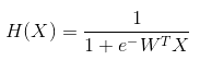
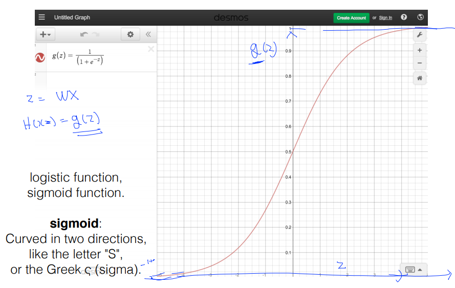
- softmax : ① sigmoid와 마찬가지로 0과 1사이의 값으로 변환, ② 변환된 결과에 대한 합계가 1이 되도록 해줌(≒ 확률)
- one-hot encoding : softmax로 구한 값 중에서 가장 큰 값을 1로, 나머지를 0으로 만듦 (tensorflow의 argmax 함수 이용)
4. Cost function (=cross-entropy)
- S(Y) = sotmax가 예측한 값
- L = 실제 Y의 값
- Cost function = (sotmax가 예측한 값)과 (실제 Y의 값)의 차이를 계산 = Distance(S, L)
- Loss(=cost=error) = D(S,L)의 평균
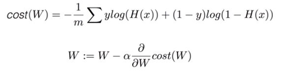
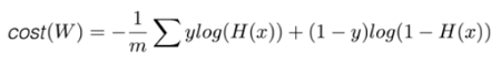
- Gradient descent 알고리즘 = 미분을 통해 최소비용 찾기
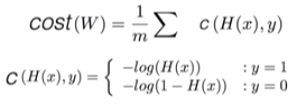
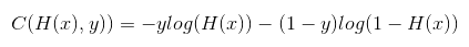
5. Logistic cost VS cross entropy
- Logistic regression의 cost 함수 = Multinomial classification의 cross-entropy cost 함수
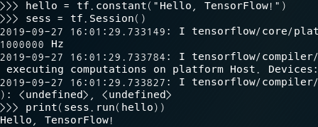
6. TensorFlow로 Softmax Classification의 구현
- cost = tf.reduce_mean(-tf.reduce_sum(Y*tf.log(hypothesis),axis=1))
- optimizer = tf.train.GradientDescentOptimizer(learning_rate=0.1).minimize(cost)
6-1. code 구현
import tensorflow as tf
tf.set_random_seed(777 ) # for reproducibility
x_data = [[1 , 2 , 1 , 1 ],
[2 , 1 , 3 , 2 ],
[3 , 1 , 3 , 4 ],
[4 , 1 , 5 , 5 ],
[1 , 7 , 5 , 5 ],
[1 , 2 , 5 , 6 ],
[1 , 6 , 6 , 6 ],
[1 , 7 , 7 , 7 ]]
y_data = [[0 , 0 , 1 ],
[0 , 0 , 1 ],
[0 , 0 , 1 ],
[0 , 1 , 0 ],
[0 , 1 , 0 ],
[0 , 1 , 0 ],
[1 , 0 , 0 ],
[1 , 0 , 0 ]]
X = tf.placeholder(" float" None , 4 ]) # x_data와 같은 크기의 열 가짐. 행 크기는 모름.
Y = tf.placeholder(" float" None , 3 ])
nb_classes = 3
W = tf.Variable(tf.random_normal([4 , nb_classes]), name = ' weight'
b = tf.Variable(tf.random_normal([nb_classes]), name = ' bias'
# tf.nn.softmax computes softmax activations
# softmax = exp(logits) / reduce_sum(exp(logits), dim)
hypothesis = tf.nn.softmax(tf.matmul(X, W) + b)
# Cross entropy cost/loss
cost = tf.reduce_mean(- tf.reduce_sum(Y * tf.log(hypothesis), axis = 1 ))
optimizer = tf.train.GradientDescentOptimizer(learning_rate = 0.1 ).minimize(cost)
# Launch graph
with tf.Session() as sess:
sess.run(tf.global_variables_initializer())
for step in range (2001 ):
_, cost_val = sess.run([optimizer, cost], feed_dict = {X: x_data, Y: y_data})
if step % 200 == 0 :
print (step, cost_val)
print (' --------------'
# Testing & One-hot encoding
a = sess.run(hypothesis, feed_dict = {X: [[1 , 11 , 7 , 9 ]]})
print (a, sess.run(tf.argmax(a, 1 )))
print (' --------------'
b = sess.run(hypothesis, feed_dict = {X: [[1 , 3 , 4 , 3 ]]})
print (b, sess.run(tf.argmax(b, 1 )))
print (' --------------'
c = sess.run(hypothesis, feed_dict = {X: [[1 , 1 , 0 , 1 ]]})
print (c, sess.run(tf.argmax(c, 1 )))
print (' --------------'
all = sess.run(hypothesis, feed_dict = {X: [[1 , 11 , 7 , 9 ], [1 , 3 , 4 , 3 ], [1 , 1 , 0 , 1 ]]})
print (all , sess.run(tf.argmax(all , 1 )))
6-2. 결과값
(0, 6.926112)
7. TensorFlow로 Fancy Softmax Classifier 구현 (cross_entropy, one_hot, reshape)
7-1. softmax_cross_entropy_with_logits
- logits(=score) = tf.matmul(X, W) + b
- hypothesis = tf.nn.softmax(logits)
7-2. tensorflow 구현 (tensorflow 내장함수 이용)
# Cross entropy cost/loss
cost = tf.reduce_mean(-tf.reduce_sum(Y*tf.log(hypothesis), axis=1)
# Cross entropy cost/loss
cost_i = tf.nn.softmax_cross_entropy_with_logits (logits=logits, labels=Y_one_hot)
cost = tf.reduce_mean(cost_i)
7-3. 예제 : 동물 분류(Animal classification)
- tf.one_hot : one_hot을 사용하게 되면 하나의 차원의 수를 높여준다. 예를들어 [0, 3]의 행렬을 [[1000000], [0001000]]의 식으로 만들어 주게 된다.
- tf.reshape : 늘어난 차원의 수를 다시 줄이기 위해, reshape 함수를 이용한다.
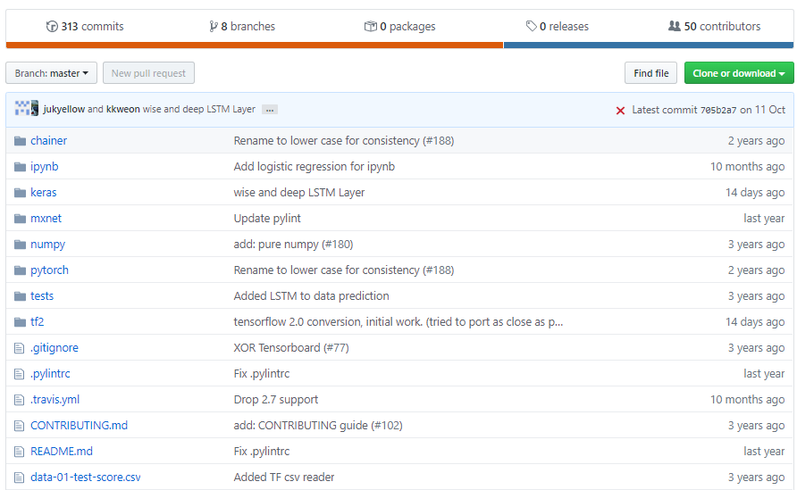
- zoo.data : https://archive.ics.uci.edu/ml/machine-learning-databases/zoo/zoo.data
불러오는 중입니다...
- 전체 소스코드
import tensorflow as tf
import numpy as np
tf.set_random_seed(777 ) # for reproducibility
# Predicting animal type based on various features
xy = np.loadtxt(' data-04-zoo.csv' delimiter = ' ,' dtype = np.float32)
x_data = xy[:, 0 :- 1 ]
y_data = xy[:, [- 1 ]]
print (x_data.shape, y_data.shape)
'''
(101, 16) (101, 1)
'''
nb_classes = 7 # 0 ~ 6
X = tf.placeholder(tf.float32, [None , 16 ]) # x_data(동물 형질 항목)의 개수
Y = tf.placeholder(tf.int32, [None , 1 ]) # 0 ~ 6
Y_one_hot = tf.one_hot (Y, nb_classes) # one hot, 차원의 수가 1차원 증가함
print (" one_hot:"
Y_one_hot = tf.reshape (Y_one_hot, [- 1 , nb_classes])
print (" reshape one_hot:"
'''
one_hot: Tensor("one_hot:0", shape=(?, 1, 7), dtype=float32)
reshape one_hot: Tensor("Reshape:0", shape=(?, 7), dtype=float32)
'''
W = tf.Variable(tf.random_normal([16 , nb_classes]), name = ' weight'
b = tf.Variable(tf.random_normal([nb_classes]), name = ' bias'
# tf.nn.softmax computes softmax activations
# softmax = exp(logits) / reduce_sum(exp(logits), dim)
logits = tf.matmul(X, W) + b
hypothesis = tf.nn.softmax(logits)
# Cross entropy cost/loss
cost = tf.reduce_mean(tf.nn.softmax_cross_entropy_with_logits_v2(logits = logits,
labels = tf.stop_gradient([Y_one_hot])))
optimizer = tf.train.GradientDescentOptimizer(learning_rate = 0.1 ).minimize(cost)
prediction = tf.argmax(hypothesis, 1 ) # probability -> 0~6
correct_prediction = tf.equal(prediction, tf.argmax(Y_one_hot, 1 ))
accuracy = tf.reduce_mean(tf.cast(correct_prediction, tf.float32))
# Launch graph (학습)
with tf.Session() as sess:
sess.run(tf.global_variables_initializer())
for step in range (2001 ):
_, cost_val, acc_val = sess.run([optimizer, cost, accuracy], feed_dict = {X: x_data, Y: y_data})
if step % 100 == 0 :
print (" Step: {:5 } \t Cost: {:.3f } \t Acc: {:.2% } "
# Let's see if we can predict
pred = sess.run(prediction, feed_dict = {X: x_data})
# y_data: (N,1) = flatten => (N, ) matches pred.shape
for p, y in zip (pred, y_data.flatten()):
print (" [{} ] Prediction: {} True Y: {} " == int (y), p, int (y)))
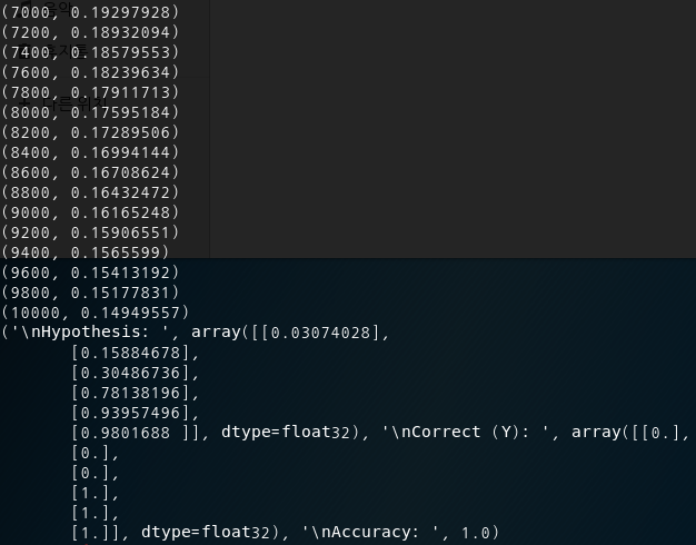
- 결과값
Step: 0 Cost: 5.480 Acc: 37.62%